Getting started
Contents
Getting started
Obtaining the software
To get started using MKMCXX, you need to download the software package and unpack it on your machine. The package contains a single executable file. For windows, this file is called "mkmcxx.exe", for Unix this is simply "mkmcxx".
In addition to the software, you also need to obtain a text editor. On Unix systems, typically vim or nano is installed. For Windows, we recommend using Notepad++.
Running the program
Performing a simulation works somewhat different on Windows as compared to Unix. Please read the respective instructions below.
Windows
On Windows, you can perform simulations by placing these in separate folders and executing a batch file. To perform the example simulation, go to the folder where you have unpacked the software package. Open the folder place_different_runs_here and thereafter the folder example. Inside this folder, there is a file called run.bat; double-click on this file and the simulation should start.
Redistributables
If you get the error "VCRUNTIME140.dll was not found", most likely the MSVC redistributables are not installed on your machine. You can download these using the link below:
https://www.microsoft.com/en-us/download/details.aspx?id=52685
Unix
On Unix systems, simulations are typically performed using the command line. Open a terminal and go to the root folder of the MKMCXX package. In this folder, you will see a directory named bin and a directory named example. Go to the example directory and execute the program as follows:
../bin/mkmcxx -i input.mkm
Viewing the results
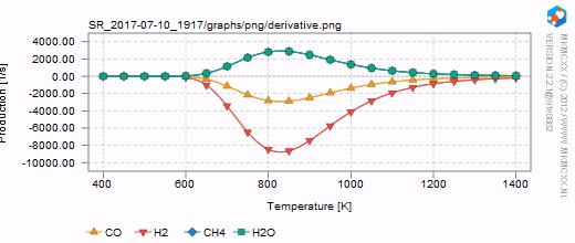
The results of the simulation are written in a separate folder. The name of the folder starts with "SR_", indicative for a sequencerun. Upon opening the SR_*** folder, you will see a list of folders for each temperature at which a simulation has been performed as well as a graphs and range folder. In the graph folder, you can find automatically generated graphs of your simulation. In the other folders, you will find the corresponding data files of your simulation. Below, two graphs are shown that can be found in the graphs/range.

