My first simulation
Overview
In this tutorial, we are going to construct a simple microkinetic simulation for the surface catalyzed conversion of A to B.
Input file
We need to construct an input file with A, A*, B*, B, and * as the main components. A can adsorb on the catalytic surface, thereafter A* is converted to B* and finally released as B to the gas phase. The gas phase concentration of A is set to unity, whereas the gas phase of B is set to 0 to model an initial rate experiment. The pressure is set to 1 bar and we perform simulations between 400K and 1200K with 100K intervals. Detailed information on how an input file is constructed can be found here.
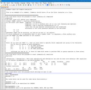
The input file is given below. We have provided additional comments to explain briefly what each settings does. You can copy the input file to your text editor and place the file in a separate directory. (see below)
# Example input for simple simulation
#
# This is an example of a comment. Comments should have a # as the first character on a line.
#
##############################################
# the line below tells the program to start indexing all compounds
&compounds
# the next lines will define your compounds
# format: NAME; isSite? ; starting concentration
# So the first line reads: 	Compound 1 is called A
#							Compound 1 is not a surface site (so it is a non changing gas species)
#							Compound 1 has a starting concentration of 1.0
#							(note that the gas species concentrations are normalized
#							according to the total pressure defined in the settings)
A;  		0;  1.0
B;  		0;  0.0
# Adsorbent names can be anything, as long as you put a 1 as isSite?.
# To avoid confusion it is generally best to use a symbol like * to represent a free surface site
# and use NAME* for NAME adsorbed on the surface.
A*;         1;  1.0
B*;         1;  1.0
*;  		1;  1.0
#
# Note: If you have set TDRC = 1, then you also need to specify which compounds are going to be evaluated.
#		You do this by adding an extra parameter.
#		CO*; 		1; 	0		<-- No TDRC performed
#		H*; 		1; 	0;	1   <-- TDRC performed
#		C*; 		1; 	0;	0	<-- No TDRC performed
#
#		(although you can do it, it does not make much sense to perform TDRC on gasous species or free sites)
#################################
# the line below tells the program to start indexing all reactions
&reactions
#
# adsorptions / desorptions - Note that adsorptions and desorption can also be done with Arhenius (AR) equations
# it is however recommended to use Hertz-Knudsen (HK)
#										 m^2		amu		K	sigma	sticking	J/mol
HK; {A}	+ 	 {*} 	=>   {A*};		1e-19;		28;	  2.73;		1;	1;			120e3
HK; {B}	+ 	 {*} 	=>   {B*};		1e-19;	 	 2;		88;		2;	1;	 		 80e3
# Surface reactions
#						vf		 vb		Eaf		Eab
AR; {A*} 	=> {B*};	6e11;	4e12;	65e3;	90e3
#################################
# the lines below tell the program which settings we want to use
&settings
TYPE = SEQUENCERUN
PRESSURE = 10
#
#DEBUG = 1
#Enables debug messages. Also produces some data on relative derivatives (dydt/y) to check for convergence (Default = 0)
#
#################################
# the lines below tell the program which runs we want to perform
&runs
#
# Temp;	Time;	AbsTol;	RelTol
400;	1e8;	1e-12;	1e-12
500;	1e4;	1e-12;	1e-12
600;	1e1;	1e-12;	1e-12
700;	1e1;	1e-12;	1e-12
800;	1e1;	1e-12;	1e-12
900;	1e1;	1e-12;	1e-12
1000;	1e1;	1e-12;	1e-12
1100;	1e1;	1e-12;	1e-12
1200;	1e1;	1e-12;	1e-12
1300;	1e1;	1e-12;	1e-12
1400;	1e1;	1e-12;	1e-12
#
# Note: You can also omit the tolerances. Then the default tolerances will be used. For example:
#		400;	1e1
#			 ^- will execute a run at 400K for 1e10 seconds at AbsTol = 1e-12 and RelTol = 1e-8
Executing the simulation
Copy the text of in the input file to your text editor (see image). Here, we have used Notepad++ as our editor, but basically any (flat-text) editor would suffice. We do not recommend using regular Windows notepad or Microsoft Word for editing these files. The former typically shows problems with newline characters and the latter is simply not made for flat texts.
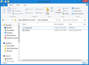
Next, create a new folder in the place_different_runs_here folder and store the file as input.mkm in that folder. Copy from the example folder run.bat to the newly created folder. The result should look like the image on the right.
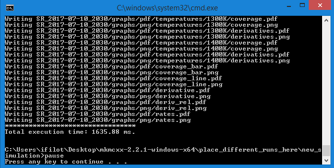
You are now all set to go and can double-click on the run run.bat file and your simulation should start. The simulation typically runs very fast and you should see an window pop-up showing something similar to the image below
Analyzing the results
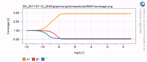
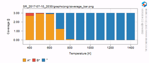
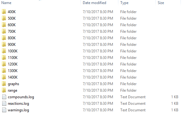
The results are written to a newly created folder which starts with SR_. SR_ stands for "sequencerun", which is the type of simulation we are conducting. If you open this folder, you should see a list of files and folders similar to the one below. In each of the temperature folders (ending with "K"), the microkinetic simulation as a function of time is given. In the range folder, the final result for each temperature is given. The results are stored in .dat which can be readily opened with Excel or some other spreadsheet utility. In the graph folder, a series of graphs, both in .PDF as well as in .PNG format can be found. On the right, a few examples of these graphs are given. You should verify that you result looks similar.
