Example selectivity
Contents
Introduction
![]() In this example, we show how to calculate selectivities and how to perform a degree of selectivity control analysis. We perform a calculation on a relatively simple chemokinetic network wherein a product A can be converted to product E or F. We wish to analyze which elementary reaction steps control the selectivity to E or F.
In this example, we show how to calculate selectivities and how to perform a degree of selectivity control analysis. We perform a calculation on a relatively simple chemokinetic network wherein a product A can be converted to product E or F. We wish to analyze which elementary reaction steps control the selectivity to E or F.
Input
In this example, the following input file is used:
&compounds
A;		0;	1
E;		0;	0
F;		0;	0
A*;		1;	0 ; 1
B*;		1;	0 ; 1
C*;		1;	0 ; 1
D*;		1;	0 ; 1
E*;		1;	0 ; 1
F*;		1;	0 ; 1
*;		1;	1.0
&reactions
#						m^2		amu			K	sigma	sticking	J/mol
HK; {A} + {*} => {A*};	1e-20;	  1;	   1;	 1;		1;			 80e3 ; 1
HK; {E} + {*} => {E*};	1e-20;	  1;	   1;	 1;		1;			 80e3 ; 1
HK; {F} + {*} => {F*};	1e-20;	  1;	   1;	 1;		1;			 80e3 ; 1
#									vf		vb		Eaf		Eab
AR; {A*}	     => {B*};			1e13;	1e13;	 90e3;	 90e3 ;1
AR; {B*}	     => {C*};			1e13;	1e13;	 80e3;	 90e3 ;1
AR; {B*}             => {D*};	1e13;	1e13;	 70e3;	 80e3 ;1
AR; {C*}	     => {E*};			1e13;	1e13;	 70e3;	120e3 ;1
AR; {D*}	     => {F*};			1e13;	1e13;	 70e3;	 90e3 ;1
&settings
TYPE = SEQUENCERUN
PRESSURE = 1
REAGENTS = {A}
KEYCOMPONENTS = {F}
EACT=1
ORDERS=1
DRC=1
TDRC=0
DEBUG=1
USETIMESTAMP=0
&runs
300;	1e6;	1e-10;	1e-10
350;	1e6;	1e-10;	1e-10
400;	1e6;	1e-10;	1e-10
450;	1e5;	1e-10;	1e-10
500;	1e4;	1e-10;	1e-10
550;	1e3;	1e-10;	1e-10
600;	1e2;	1e-10;	1e-10
650;	1e1;	1e-10;	1e-10
700;	1e1;	1e-10;	1e-10
750;	1e1;	1e-10;	1e-10
800;	1e0;	1e-10;	1e-10
850;	1e0;	1e-10;	1e-10
900;	1e0;	1e-10;	1e-10
950;	1e0;	1e-10;	1e-10
1000;	1e0;	1e-10;	1e-10
1100;	1e0;	1e-10;	1e-10
1200;	1e0;	1e-10;	1e-10
1300;	1e0;	1e-10;	1e-10
1400;	1e0;	1e-10;	1e-10
1500;	1e0;	1e-10;	1e-10
1600;	1e0;	1e-10;	1e-10
1700;	1e0;	1e-10;	1e-10
1800;	1e0;	1e-10;	1e-10
1900;	1e0;	1e-10;	1e-10
2000;	1e0;	1e-10;	1e-10
Running the calculation
The first step is to perform a regular calculation.
./mkmcxx -i input.mkm
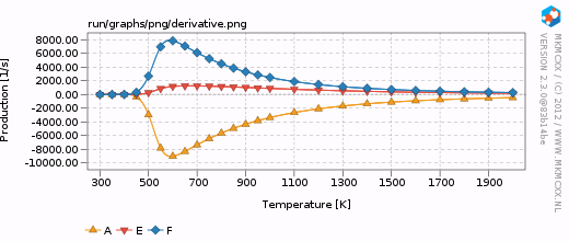
This results in the creation of a run folder wherein all the raw data is written. A plot of the turn-over frequencies is given on the right. We can easily see that there is a distinct selectivity pattern for F over E.
Performing the selectivity analysis
From the above calculation, we have seen that products E and F are both presents at all temperatures. Here, we wish to calculate the selectivity towards E and F using A as our key component. To do so, we have to add the following lines to our input file:
&selectivity
species_balance; {A}; {E},{F}
If we would now rerun the simulation, we would obtain the graphs we are interested in. However, all the data relevant to calculate the selectivity and the degree of selectivity control is already done in the previous calculation and it would be a waste of time to re-calculate these. Luckily, we can make use of a short-cut. In every calculation wherein a DRC analysis is performed, the raw data is written to a file termed drcrates.bin. We are going to load the rates and the drc analysis of the previous calculation from this file and perform the selectivity analysis on this data. The command to do so is as follows:
./mkmcxx -i input.mkm -o run/ -s
Note that the first part of the command is the same as for a regular calculation. We have added two additional directives, -o run and -s. The first directive tells the program to look for drcrates.bin in the run folder. The second directive indicates that we wish to perform a sensitivity analysis.
The result should look something like this
Writing graphs for sensitivity analysis...
Writing run/graphs/pdf/selectivity_bar_species_balance.pdf
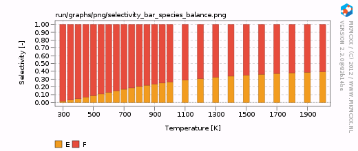
Writing run/graphs/png/selectivity_bar_species_balance.png
Writing run/graphs/pdf/selectivity_line_species_balance.pdf
Writing run/graphs/png/selectivity_line_species_balance.png
Writing run/graphs/pdf/dsc_species_balance_E.pdf
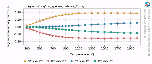
Writing run/graphs/png/dsc_species_balance_E.png
Writing run/graphs/pdf/dsc_species_balance_F.pdf
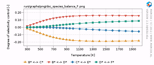
Writing run/graphs/png/dsc_species_balance_F.png
For each line in the selectivity block, a bar and a line graph for the selectivity is made. Furthermore, for each product in these blocks, an additional degree of selectivity control graph is made. The corresponding graphs are shown on the right.
In our simple chemokinetic network, reactant A could either be converted in product E or product F. Hence, a reaction that facilitates the formation of E, would result in less formation of F and vice versa. Consider now the two degree of selectivity control graphs on the right. If an elementary reaction step favors formation of E over F, then that elementary reaction step has a positive DSC coefficient for E and a negative DSC coefficient for F. Logically, if our network only has two possible products, then the result of the DSC analysis of E is the mirror image of the DSC analysis of F. This is the reason that the two DSC graphs are mirrored in the x-axis with respect to each other.
Concluding remarks
If you know in advance what kind of selectivity analysis you wish to perform, you can already place the &selectivity block in the initial calculation and the graphs are automatically generated. The advantage of the short-cut as mentioned above is that if you make mistakes or if you want to add different selectivity analyses (i.e. for other compounds), you can easily add these and perform a fast re-run to generate the relevant graphs.


